Project Objective

Cookie Cats is a hugely popular mobile puzzle game. As players progress through the game they will encounter gates that force them to wait some time before they can progress or make an in-app purchase. In this project, we will analyze the impact on player retention when the first gate in Cookie Cats was moved from level 30 to level 40.

Analytical Objective

Test hypothesis to analyze if moving the first gate from level 30 to 40 will increase retention rate and total number of game rounds played.

Dataset Used

Mobile Games A/B Testing with Cookie Cats Project data downloaded from https://www.datacamp.com/projects/184
The data contains the details gameplay from 90,189 users and it contains 5 columns:

1. userid - a unique number that identifies each player.
2. version - whether the player was assigned to gate_30 or gate_40.
3. sum_gamerounds - the number of game rounds played by the player during the first week after installation
4. retention_1 - did the player come back and play 1 day after installing?
5. retention_7 - did the player come back and play 7 days after installing? When a player installed the game, he is randomly assigned to either gate_30 or gate_40 version.

Importing library and data

import numpy as np
import pandas as pd 
import seaborn as sns
import matplotlib.pyplot as plt
from scipy.stats import shapiro
import scipy.stats as stats

# Read data from csv into pandas dataframne
user_df=pd.read_csv("Project_Data.xls")

# Check dimension of data
user_df.shape

# Check data info
user_df.info()

# display first 5 rows of the data
user_df.head(5)

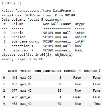
The dataset contains 5 columns as shown in the screenshot above. It seems to contain no missing values and the dtypes are appropriate.

Inspect the data and resolve data quality issues

# Check for missing values in the data
user_df.isnull().sum()

# Check if there is any duplicate userid
user_df["userid"].nunique()

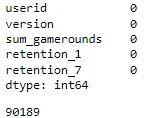
From the above functions, it can be confirmed that there is no missing or duplicate values in the dataset. Next, let’s look at the distribution of the data.

user_df['sum_gamerounds'].describe()

count 90189.000000
mean 51.872457
std 195.050858
min 0.000000
25% 5.000000
50% 16.000000
75% 51.000000
max 49854.000000

The above output indicates a high standard deviation with number of gamerounds played ranging from 0 to 49854.
Interestingly, 75% of users played 51 levels or less but the maximum number of levels played is 49854. We further investigate this to understand the data more.

buckets = [0,1,6,11,31,101,501,1001,max(user_df['sum_gamerounds'])+1]
user_df['gamerounds_cut'] = pd.cut(user_df['sum_gamerounds'],buckets,right=False)
user_df['gamerounds_cut'].value_counts(normalize=True).sort_index()

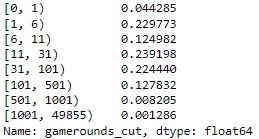
The above code splits the number of gamerounds into buckets to display a more detailed segregation based on number of gamerounds played. The buckets widths are self-defined, hence it can be adjusted according to any threshold that is meaningful to the viewers. We have segregated them into 8 buckets.

From the above output, we observe the below:

Observation 1

4.4% of users (3,994 users) downloaded the games but did not play a single level.
There are several possible explanations to this:

1. Users have yet to start the game
2. Users dislike the interface/design and decided not to play
3. Users face technical issues with the gameplay

Observation 2

22.9% of users (20,723 users) played 5 levels or less.
This could mean that:

1. Users started playing but did not find the game attractive
2. Users did not have time to play during the week

user_df[(user_df['sum_gamerounds']>0) & (user_df['sum_gamerounds']<6)][['retention_1','retention_7']].value_counts(normalize=True)

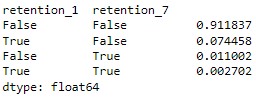
We investigate further and realise that 91.18% of users who played 5 levels or less did not play the game again after day 1 of download.

Both observation 1 and 2 could be a normal trend in mobile game industry, where users are spoilt for choices and often download multiple games at once just to try out. It is recommended to compare to these figures to previous game launches’ downloads and retention trends. Further user research can also be done to understand user experience so as to identify potential improvement that can increase retention.

Observation 3

The output above shows that the median number of gamerounds played is 16 rounds, and 75% of users played 51 rounds or less. However, the maximum number of gamerounds played is 49854.

user_df.plot(y='sum_gamerounds',figsize = (15,6), color = "#ff9900", xlabel="Index",ylabel="Gamerounds")
plt.title("Total Gamerounds Played",fontweight ='bold', fontsize = 15)
plt.savefig(fname='chart1.jpg')
plt.show()

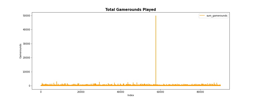
A quick plot shows that the maximum number of gamerounds seem to be an outlier.

# remove outlier 
user_df = user_df.drop(user_df[user_df['sum_gamerounds']>10000].index)

#Plot the graph again after removing the outlier
user_df.plot(y='sum_gamerounds',figsize = (15,6), color = "#ff9900")
plt.title("Total Gamerounds Played",fontweight ='bold', fontsize = 15)
plt.xlabel("Index")
plt.ylabel("Gamerounds")

plt.show()

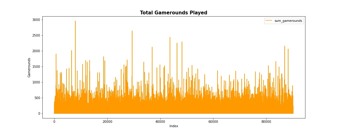This is how the chart looks after removing the outlier row.

Compare Gate_30 and Gate_40 Version

Let’s compare the retention rate and total gamerounds played for both version.

# creating new df showing retention and gamerounds played for both version
df = user_df.groupby('version')[['retention_1','retention_7','sum_gamerounds']].sum()
df.loc['total', :] = df.sum()

df1 = user_df.groupby('version')[['retention_1','retention_7','sum_gamerounds']].mean().apply(lambda x: round(x,4))
df1.loc['total', :] = round((df.loc['total']/len(user_df)),4)
df1[['retention_1','retention_7']] = df1[['retention_1','retention_7']].apply(lambda x: x*100)
df1.rename(columns={"retention_1": "retention_1(%)", "retention_7": "retention_7(%)", 'sum_gamerounds': 'sum_gamerounds (mean)'},inplace=True)

df_pct = pd.merge(df, df1, on='version')
df_pct.sort_index(axis=1, inplace=True)
df_pct

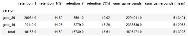
The table above shows the number of users retained after 1 day, 7 days and the total & mean gamerounds played for each version.
We observe the below:

Overall

1. Retention rate after 1 day = 44.52%
2. Retention rate after 7 days = 18.61%
3. Average number of gamerounds played = 51.32

Compare Gate_30 and Gate_40 Version

1. Version gate_30 has higher retention rate after 1 day - 44.82% vs 44.23% for Version gate_40
2. Version gate_30 has higher retention rate after 7 days - 19.02% vs 18.20% for Version gate_40
3. Users in Gate_30 version played slightly more gamerounds (51.34) on average than users in Gate_40 version (51.30).

Hypothesis Testing

Before further analysis, we want to find out if the number of gamerounds played under the 2 versions are statistically different using statistical tests.

# Split the data of 2 versions into group A and group B
group_A = pd.DataFrame(user_df[user_df.version=="gate_30"]['sum_gamerounds'])
group_B = pd.DataFrame(user_df[user_df.version=="gate_40"]['sum_gamerounds'])

To identify the appropriate test method to test the means of 2 groups, we first check if the distribution of the sum of gamerounds for both groups conform to normal distribution.

Shapiro Test

We perform Shapiro Test to test the normality of distribution. Hypothesis is defined as below:

H0: Distribution is normal
H1: Distribution is not normal

alpha = 0.05
#test for group_A
stats.shapiro(group_A['sum_gamerounds'])

#test for group_B
stats.shapiro(group_B['sum_gamerounds'])

Output: ShapiroResult(statistic=0.4825654625892639, pvalue=0.0)

At 95% confidence level, as p value for both groups A and B are less than 0.05, we reject the null hypothesis and infer that distributions for both groups are not normally distributed.

Levene's Test

We then perform Levene’s Test to find out if the variance of both groups are equal. Hypothesis is defined as below:

H0: Both groups have equal variances
H1: Both groups do not have equal variances

alpha = 0.05
stats.levene(group_A['sum_gamerounds'],group_B['sum_gamerounds'])

Output: LeveneResult(statistic=0.07510153837481241, pvalue=0.7840494387892463)

At 95% condidence level, there is insufficient statistical evidence to reject the null hypothesis (p value > alpha), hence, we can infer that the two groups have equal variances.

Mann-Whitney U test

As both group A & B do not conform to normal distribution but have equal variance, we use non-parametric test (Mann-Whitney U test / Wilcoxon rank-sum test) to test the hypothesis.

H0: Both Group A and B have equal mean number of gamerounds played.
H1: Both Group A and B do not have equal mean number of gamerounds played.

alpha = 0.05
stats.mannwhitneyu(group_A['sum_gamerounds'],group_B['sum_gamerounds'])

Output: MannwhitneyuResult(statistic=1009027049.5, pvalue=0.02544577639572688)

At 95% confidence interval, as p value (0.025) is less than alpha (0.05), there is sufficient statistical evidence to reject the null hypothesis. We infer that Group A and B do not have equal mean number of gamerounds played.

Analysis and Recommendation

From the section above, we know that:

1. Version gate_30 has higher retention rate after 1 day - 44.82% vs 44.23% for Version gate_40
2. Version gate_30 has higher retention rate after 7 days - 19.02% vs 18.20% for Version gate_40
3. Users in Gate_30 version played slightly more gamerounds (51.34) on average than users in Gate_40 version (51.30).

To add on, we compute the maximum number of gamerounds played by users under each group:

max_gamerounds = user_df.groupby('version')['sum_gamerounds'].max()
max_gamerounds

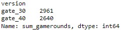
The above output shows that the maximum gamerounds played by players in Version gate_30 is more than the max gamerounds in Version gate_40 (2961 vs 2640).

Based on these 3 findings, it is wiser to keep the gate at level 30 since version gate_30 produces higher retention and more gamerounds played on average.

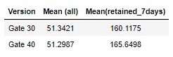
However, we also noticed that even though Gate_30 version has higher mean gamerounds played, if we filter only players who come back to play after 7 days (retention_7==True), version Gate_40 has higher mean gamerounds played.

user_df_retained7 = user_df[user_df['retention_7'] == True]
user_df_retained7.groupby('version')['sum_gamerounds'].mean()

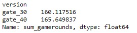
Comparision of gamerounds played for both groups (all users who downloaded vs users retained after 7 days)

Whether to place the gate at level 30 or 40 depends on the business objective. If the aim is to retain as many users as possible at day 7, then the gate should be kept at level 30. Nevertheless, if the aim is to generate higher revenue through in-app purchases, the analysis focus might be shifted to more gamerounds played, excluding players with low gamerounds, as players in higher levels might have better chance on spending on in-app purchase. It is recommended to also include other dimensions (such as in-app purchase spending, age of players etc) into the analysis if the aim is about generating higher revenue.